
Crypto Price Modelling Basics
In this piece we shall aim to cover some very high level basics on statistical modelling of asset prices in order to relate some analogies into our expectations of the price of CSPR.
Normal Returns vs Lognormal Prices
Before we begin, lets first cover a couple of common distributions used in financial modelling. For those who are not familiar with distributions, they are simply graphs which show what a result will likely be if its picked at random from a process which follows the distribution. The higher the point on the chart the more likely that value (on the x-axis will be picked).
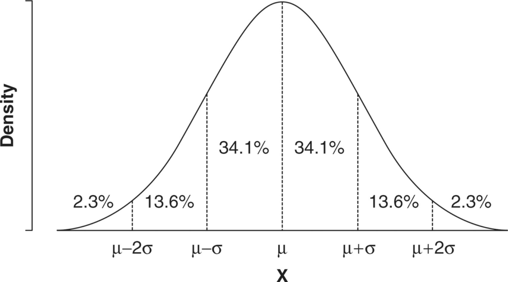
- Normal distribution – a symmetrical bell shaped distribution is used typically used to model returns. When centred around zero (i.e. the peak of the chart is at 0), the distribution will show an equal probability of having a negative or positive return. This is because there is equal area under the chart in the regions to the left (<0) as there is to the right (>0) of the centre. If a random process follows this distribution, it means that, on average the value of the process will be the centre of the distribution (as this has the highest point on the chart), i.e. the same as previous. The further out to the right (positive) and left (negative), you will note the high of the chart decreases in height, meaning that these values are less likely (i.e. extreme returns for the next period are less likely than smaller returns or flat return). If we consider the mean to be zero, and the chart to represent ‘next period returns’, then we can say there is the same likelihood of a positive return in the next period as there is a negative return. The two key characteristics of a normal distribution are the (1) mean and (2) standard deviation. As discussed, the mean is the centre of the chart whereas the standard deviation is the distance from the centre, equal in both directions, such that the area under the chart is equal to 68.2% of the total area under the chart.
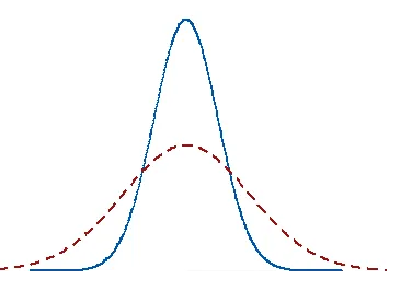
We can move the distribution by changing the mean (i.e. the centre of the chart, and we can also flatten the peak by adjusting the standard deviation. Increasing the standard deviation will result in a wider more flatter chart (please see chart below). When representing asset returns, a larger standard deviation will indicate greater volatility as there is greater change of extreme returns and less chance of smaller returns. The red distribution below can be considered more volatile than the blue.
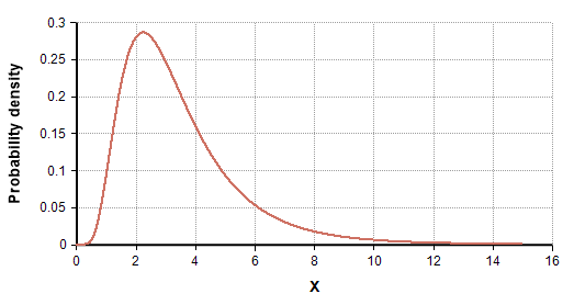
- Lognormal distribution – You will note that we are very careful to only talk about ‘returns’ when discussing the normal distribution – this is because returns can be both positive and negative. Prices on the other hand cannot be negative and so are modelling using a lognormal distribution (as been below)
Asset Process
We shall overly simplify some complex topics in order to keep this article concise. We can think of asset price growth as consisting of 2 parts (1) the average expected growth plus (2) the volatility in the growth. We are all likely familiar with the highly volatile nature of Bitcoin and also how it has in general grown in value in the last 10 year. On average the price has risen but when looking at specific periods of time, we can note extremely sharp declines or gains Within asset modelling these two properties help us simulate future potential prices using the following equation (Geometric Brownian Motion). Effectively what the equation is showing is that the change in price (left of equation), is equal to the sum of the two components.
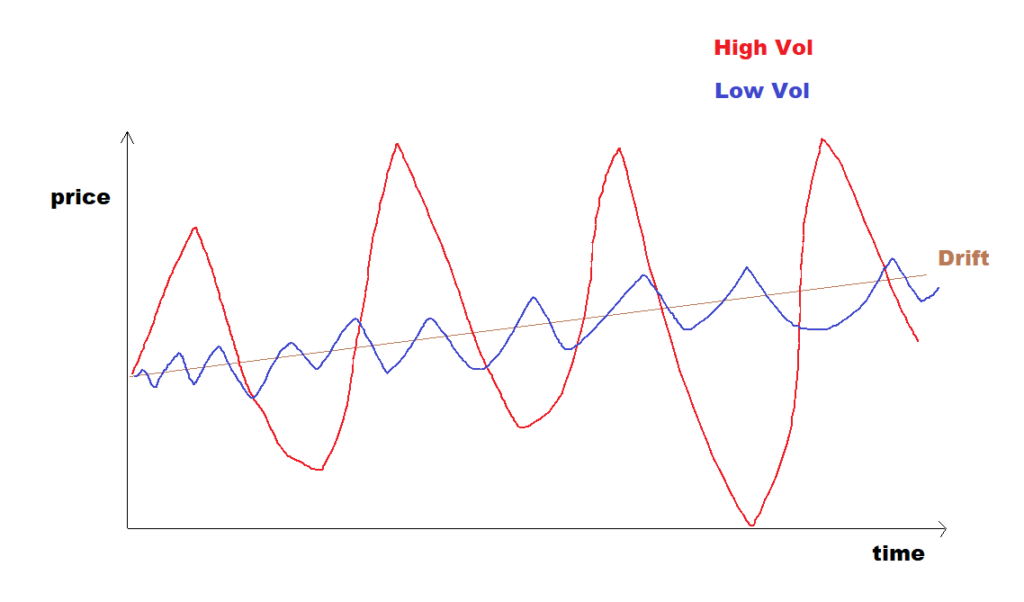
- Drift – or average growth. We can think of the drift as an upward sloping straight line (the long term average growth in prices)
- Diffusion – or uncertainty (also known as volatility). We can think of this as a normal distribution, where the outcome can be positive or negative with a magnitude lined to the standard deviation of the normal distribution
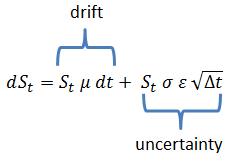
We can therefore think that tomorrows price will be made up of the drift plus a random positive or negative amount based upon the diffusion (or volatility). The size of the random move will be based upon a normal distribution and the bigger the standard deviation in the normal distribution, the bigger this diffusion component will be to the price.
Below is an over simplified illustration of two assets with the same drift but differing volatility. I have over simplified this for ease of explanation but in reality, observing the GBM equation you can see that there is a dependency on current price when estimating the next price meaning price will diverge from the line that I have named ‘drift’ below.
Additional Considerations
So far we have discussed volatility as being symmetrical (i.e. same likelihood of being positive as being negative), and that asset prices can be forecast using only two components (1) drift and (2) volatility. In reality of course, asset prices and market are considerably more complex than this. Some real world components to consider:
- Change in fundamentals of the asset (idiosyncratic risk)
- Change in market (systematic risks)
- Correlation between assets
- Price support levels
Correlations can be modelled using historical data and both idiosyncratic/systematic risks can be incorporated into the process by applying random jumps into the process to simulate these.
Additionally we can consider regimes, mean-reverting, momentum or both, using tools such as
- Pattern recognition on the Fractal Market Hypothesis or wave theory such as that of the Elliot wave theory
- Augmented Dicky Fuller test (non stationary time series)
- Central Limit Test (stationary time series)
We can now note how complex it therefore becomes to understand the dynamics of the market from a purely modelling points of view.
To further add, correlation can also exhibit a complex non-symmetricality, whereby prices in one asset are correlated to another only in one direction. This is prominent within the crypto space where newly issued tokens will have less price history and therefore fewer support levels meaning they are more susceptible to more severe drops in price when Bitcoin is in a downtrend. Temporary upticks in Bitcoin during this downtrend will rarely manifest as upticks in the newly launched alt coin. Additionally when Bitcoin is in an ascending phase, newly issued alts will be more susceptible to greater price rises, and will be resistant to pullback on down ticks in Bitcoin. We have seen this phenomena during the 2020 bull market where only after Bitcoin established itself in a definite bull run, did the more newly issued alt began to climb in value. On the bitcoin downturn, these alts suffered greater price corrections and the tokens launched in 2021 rarely experienced upticks in line with those seems in Bitcoin during its decline. This can be seen as skewed volatility, i.e. no longer a symmetrical normal distribution, but tilted in one direction depending on the medium term bitcoin trend.
With regard to what we have discussed in this article we can split the crypto token population into 3 primary categories:
- High volatility, negative drift: these are typically the highly speculative meme coins which exhibit large pumps and dumps with no real long term value or utility. Speculating in these tokens can be highly rewarding due to the volatility but the negative drift implies they are not suitable for long term holding. Additionally there exists sizable risks of being wiped due to the negative drift, where holding will not recovery losses if a trade is poorly timed.
- Newly issued tokens with strong fundamentals: These will exhibit a high long term drift component but will also begin life with very high skewed volatility dependent on the regime which Bitcoin is following at the time of issuance.
- Established tokens with strong fundamentals: These will have typically less potential for exaggerated price rises in comparison with more newly issued tokens however will also experience less volatility due to support levels being built into the price from historical trading. The skew on these tokens will also be less and more directly correlated with Bitcoin (for now)
CSPR falls into the second category due to its strong fundamentals. However it is also exposed to higher volatility and will be more negatively impacted with a declining Bitcoin due to the skew. We at Ghost Staking however believe that Bitcoin will not fall substantially further than the its current correction levels and so believe here is very case for investing in CSPR in its current price level.
Disclaimer: This article is written for the purposes of research and does not constitute financial advice or a recommendation to buy.